template-example
template-example.Rmd
######### << START INPUT >> ####################################################

##### 1. Global parameters
# Number of hypotheses included in the testing strategy with FWER control
numHyp        <- 4
# Allowed one-sided FWER
alphaTotal    <- 0.025
# Number of digits to report for p-value boundaries
pdigits       <- 5
# Number of rounding digits for information fractions
idigits       <- 2
# Data availability at IA in percent relative to max
plotInPercent <- FALSE
# Time limit in plot
Tmax_atPlot   <- 60
# Study specific parameter for multiple testing procedure
mtParam       <- 0.4

##### 2. Enrollment
# (This is aux to define enrollment per hypothesis below, might need enrollment
# per hypothesis for sub-population analysis)
enrollmentAll <- tibble::tibble(stratum  = "All",
                                duration = 250*2/25,
                                rate     = 25)

##### 3. Main input tibble
# One row per hypothesis
inputD        <- tibble::tibble(
  # Hypothesis IDs
  id            = paste0("H", 1:numHyp),
  # Hypothesis tags, used in graph and output tables
  tag           = c("PFS B+", "PFS", "ORR", "PRO"),
  # The fields 'regimen', 'ep', and 'suffix' are pasted together into 'descr'
  # field for the table defining hypotheses, 'tblInput'
  regimen       = rep("DrugX" , each = numHyp),
  ep            = c("PFS", "PFS", "ORR", "PRO"),
  suffix        = c("BM+", "all", "all", "all"), # E.g., for subgroups
  # Type of hypothesis (primary or secondary)
  type          = c("primary", "primary", "secondary", "secondary"),
  # initial weights in graphical multiple testing procedure
  w             = c(1, 0, 0, 0),
  # Spending functions; use NULL if no group sequential test for Hi
  grSeqTesting  = list(
    H1 = list(sfu = gsDesign::sfPower, sfupar = 2),
    H2 = list(sfu = sfPower, sfupar = 2, nominal = 0.0001),
    H3 = NULL,
    H4 = NULL
  ),
  # 'iaSpec' and 'hypN' are uses to derive the information fractions, 'infoFr',
  # and timing,'iaTiming' (calendar time since study start), for the analyses
  # For each hypothesis, set criteria that trigger analyses through
  # list(A1_list, A2_list, ..., Aj_list), where
  # Aj_list = list(H = 1, atIF = 0.5) means that for that hypothesis analysis
  # j takes place when H1 is at 0.5 information fraction
  iaSpec        = list(
    list(A1 = list(H = 2, atIF = 0.70), A2 = list(H = 2, atIF = 1)),
    list(A1 = list(H = 2, atIF = 0.70),
         A2 = list(H = 2, atIF = 0.85),
         A3 = list(H = 2, atIF = 1)),
    list(A1 = list(H = 2, atIF = 1)),
    list(A1 = list(H = 2, atIF = 1))
  ),
  # Set total information, N, for a given hypothesis (sample size or events);
  # leave NA if 'enrollment' and 'iaSpec' would define N
  hypN          = c(NA, 350, NA, NA),
  # In some cases, would need to define 'infoFr' and 'iaTime' explicitly
  # infoFr        = list(),
  # Calendar time of analysis
  # iaTime        =  list(),
  # To define hypothesis test statistics Zi ~ N(., 1), use 'endpointParam'
  # Class of 'endpointParam' is used to derive effect delta and standardized
  # effect. Standardized effect size is used for power calculations. Several
  # options are available to set test for binary endpoints.
  endpointParam = list(
    structure(
      list(
        p1            = 0.60*log(2)/10,
        p2            = log(2)/10,
        dropoutHazard = -log(1 - 0.05)/12
      ),
      class = "tte_exp"
    ),
    structure(
      list(
        p1            = 0.70*log(2)/15,
        p2            = log(2)/15,
        dropoutHazard = -log(1 - 0.05)/12
      ),
      class = "tte_exp"
    ),
    structure(
      list(
        p1            = 0.85,
        p2            = 0.70,
        maturityTime  = 6
        ),
      class = "binomial_pooled"),
    structure(
      list(
        p1            = 0.45,
        p2            = 0.10,
        maturityTime  = 3
        ),
      class = "normal")
  ),
  # Allocation ratio; trt/control
  allocRatio    = 1,
  # Prevalence of the hypotheses
  prevalence    = c(0.66, 1, 1, 1),
  # Compute enrollment to each hypothesis using its prevalence and the
  # previously set enrollment information
  enrollment    = lapply(prevalence, function(a) {
    purrr::modify_at(enrollmentAll, "rate", ~{a*.x})
  })
)

##### 4. Define graphical testing procedure
graphProc     <- function(s, hypNames = NULL) {
  # s - split parameter
  m             <- matrix(0, numHyp, numHyp)
  m[1, 2]       <-  1
  m[2, 3]       <- 1 - s
  m[2, 4]       <- s
  m[3, 4]       <- 1
  m[4, 3]       <- 1
  if (!is.null(hypNames)) {
    colnames(m) <- rownames(m) <- hypNames
  }
  new("graphMCP", m = m, weights = inputD$w)
}
G             <- graphProc(mtParam,
                           hypNames = paste(inputD$id, inputD$tag, sep = ": "))

##### 5. Depict the graphical testing procedure (refer to ?gMCPLite::hGraph)
graphFigure   <- gMCPLite::hGraph(
  nHypotheses     = numHyp,
  nameHypotheses  = paste(inputD$id, inputD$tag, sep = ": "),
  legend.name     = "Color scheme",
  #labels          = c("Regimen1", "Regimen2"),
  #legend.position = c(.5, 0.2),
  #fill            = rep(1:2, each = numHyp/2),
  #palette         = c("cyan4", "lightblue"),
  halfWid         = 0.4,
  halfHgt         = 0.2,
  trhw            = 0.15,
  trhh            = 0.05,
  offset          = 0.2,
  size            = 4,
  boxtextsize     = 3.5,
  trdigits        = 3,
  # relative position of plots on MT graph
  x               = c(1, 3, 2, 4),
  y               = c(0, 0, -1, -1),
  alphaHypotheses = gMCPLite::getWeights(G),
  m               = gMCPLite::getMatrix(G),
  wchar           = "w"
)

######### << END INPUT >> ######################################################Multiplicity Adjustment
The multiplicity strategy follows the graphical approach for group sequential designs of Maurer and Bretz (2013) which provides strong control of type 1 error. The procedure takes into account both sources of multiplicity: multiple hypothesis tests (e.g., across primary and secondary endpoints) and multiple analyses planned for the study (i.e., interim and final analyses).
There are two key components that define this approach
- Testing algorithm for multiple hypotheses specified by the graphical representation
- Repeated testing of some hypotheses using the alpha-spending function methodology
The multiplicity strategy will be applied to the 2 primary superiority hypotheses ( PFS B+ and PFS ) and 2 key secondary superiority hypotheses ( ORR and PRO ). Table @ref(tab:inputTable) summarizes the hypotheses specifying alpha-spending functions (for hypotheses to be tested group sequentially) together with the effect sizes and planned maximum statistical information (sample size or number of events).
| Label | Description | Type | Initial weight | Group Sequential Testing | Effect size* | n† |
|---|---|---|---|---|---|---|
| H1 | PFS B+ | primary | 1 | Kim-DeMets (power), parameter = 2 | HR = 0.60 (mCntl = 10.0 mo) | 263 |
| H2 | PFS | primary | 0 | Nominal spend at IA 1, then Kim-DeMets (power), parameter = 2 | HR = 0.70 (mCntl = 15.0 mo) | 350 |
| H3 | ORR | secondary | 0 | No group sequential testing | 0.15 (85% vs 70%) | 500 |
| H4 | PRO | secondary | 0 | No group sequential testing | 0 | 500 |
| * Mean difference for binary and continouos endpoints or hazard ratio (HR) for TTE endpoints | ||||||
| † Sample size or number of events for TTE endpoints |
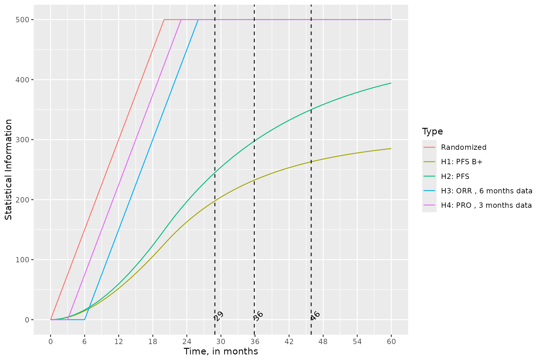
Figure @ref(fig:timelinePlot) provides details as for statistical information projected to be available (in percentage relative to maximum) versus time since the trial start by the endpoint types. The vertical lines on the figure mark times on the interim analyses.
The overall type I family-wise error rate for 4 hypotheses, over all (interim and final) analyses, is controlled to 2.5% (one-sided).
Figure @ref(fig:MTgraph) shows the graph where the hypotheses of interest are represented by the elliptical nodes. Each node has the hypothesis weight assigned to it (denoted by ). A particular value of sets the local significance level associated with that hypothesis (which is equal to 0.025). The graphical approach allows local significance levels to be recycled (along arrows on the graph) when a given hypothesis is successful (i.e., the corresponding null hypothesis is rejected) at interim or final analyses. Each arrow specifies the fraction of (by the number attached to it) to be transferred from the source node to the destination node. This “alpha-propagation” results in a corresponding increase of the local significance level of the destination node. Figure @ref(fig:MTgraph) defines the initial configuration of the local significance levels and the directed edges (arrows). Particularly, the initial weight assignment for PFS BM+ is set to 1, respectively.
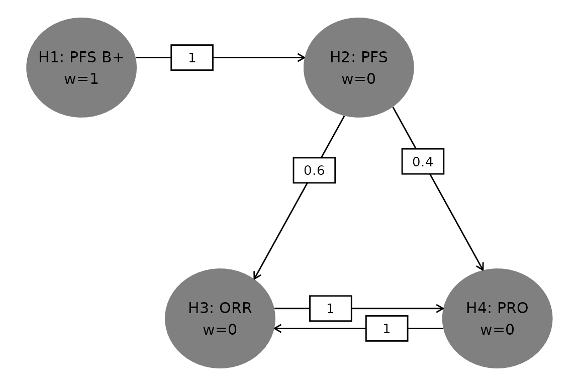
Graph Depicting Multiple Hypothesis Testing Strategy.
The testing algorithm codes a series of graph transformations which happens at each successful clearing of a hypothesis as described in Maurer and Bretz (2013). During an execution of the procedure, different scenarios as for local significance levels emerge in an iterative manner.
Interim Analyses
Table @ref(tab:iaDetailsTableA) and @ref(tab:iaDetailsTableB) summarize the the planned interim analyses.
| Hypothesis Analysis | Criteria for Conduct | Targeted Analysis Time | n† | Information Fraction |
|---|---|---|---|---|
| H1 (PFS B+) | ||||
| 1 | H2 at information fraction 0.7 | 28.93 | 198 | 0.75 |
| 2 | H2 at information fraction 1 | 45.89 | 263 | 1.00 |
| H2 (PFS) | ||||
| 1 | H2 at information fraction 0.7 | 28.93 | 245 | 0.70 |
| 2 | H2 at information fraction 0.85 | 35.88 | 298 | 0.85 |
| 3 | H2 at information fraction 1 | 45.89 | 350 | 1.00 |
| H3 (ORR) | ||||
| 1 | H2 at information fraction 1 | 45.89 | 500 | 1.00 |
| H4 (PRO) | ||||
| 1 | H2 at information fraction 1 | 45.89 | 500 | 1.00 |
| * Sample size or number of evetns for TTE endpoints | ||||
| Hypothesis | n† | Information Fraction |
|---|---|---|
| Data cut-off #1, time = 28.9, Criteria: H2 at information fraction 0.7 | ||
| H1 (PFS B+) | 198 | 0.75 |
| H2 (PFS) | 245 | 0.70 |
| Data cut-off #2, time = 35.9, Criteria: H2 at information fraction 0.85 | ||
| H2 (PFS) | 298 | 0.85 |
| Data cut-off #3, time = 45.9, Criteria: H2 at information fraction 1 | ||
| H1 (PFS B+) | 263 | 1.00 |
| H2 (PFS) | 350 | 1.00 |
| H3 (ORR) | 500 | 1.00 |
| H4 (PRO) | 500 | 1.00 |
| * Sample size or number of evetns for TTE endpoints | ||
Timelines.
Hypothesis Testing
For each hypothesis, Table @ref(tab:graphTable) gives all possible scenarios for the local significance levels in the first column, the corresponding in the second column, and listing of scenarios as for what hypothesis testing needs to be successful in the third column.
| Local alpha level | Weight | Testing Scenario |
|---|---|---|
| H1: PFS B+ | ||
| 0.025 | 1.0 | Initial allocation |
| H2: PFS | ||
| 0.025 | 1.0 | Successful H1 |
| H3: ORR | ||
| 0.015 | 0.6 | Successful H1, H2 |
| 0.025 | 1.0 | Successful H1, H2, H4 |
| H4: PRO | ||
| 0.010 | 0.4 | Successful H1, H2 |
| 0.025 | 1.0 | Successful H1, H2, H3 |
Table @ref(tab:grSeqTable) details the procedure regarding the hypothesis testing at the interim and final analyses. If for a given hypothesis group sequential testing is planned, the table provides the nominal p-value boundary derived from the given alpha-spending function and the information fractions. This boundary will be compared to the observed p-values calculated for the test statistics at the corresponding analyses. The timing of analyses is expressed in terms of statistical information fractions, i.e., current analysis information relative to the total plan information for that hypothesis test. Also, the table reports power (cumulatively over analyses) assuming hypotheses’ effect sizes from Table @ref(tab:inputTable).
| Local alpha level | Analysis | Info fraction | Nominal p-val (1-sided) | 2 x Nominal p-val | Hurdle delta | Power |
|---|---|---|---|---|---|---|
| H1: PFS B+ | ||||||
| 0.025 |
1 2 |
0.75 1 |
0.01406 0.01915 |
0.02813 0.03831 |
0.732 0.775 |
0.92 0.98 |
| H2: PFS | ||||||
| 0.025 |
1 2 3 |
0.7 0.85 1 |
1e-04 0.01806 0.01821 |
2e-04 0.03612 0.03641 |
0.622 0.784 0.8 |
0.18 0.84 0.91 |
| H3: ORR | ||||||
| 0.015 | 1 | 1 | 0.015 | 0.03 | 0.081 | 0.97 |
| 0.025 | 1 | 1 | 0.025 | 0.05 | 0.073 | 0.98 |
| H4: PRO | ||||||
| 0.010 | 1 | 1 | 0.01 | 0.02 | 0.208 | 0.94 |
| 0.025 | 1 | 1 | 0.025 | 0.05 | 0.175 | 0.97 |
Figure @ref(fig:plotSF) visualizes alpha-spending functions profiled by local significance levels available for hypotheses describing all potential scenarios needed during an execution of the multiple testing procedure.
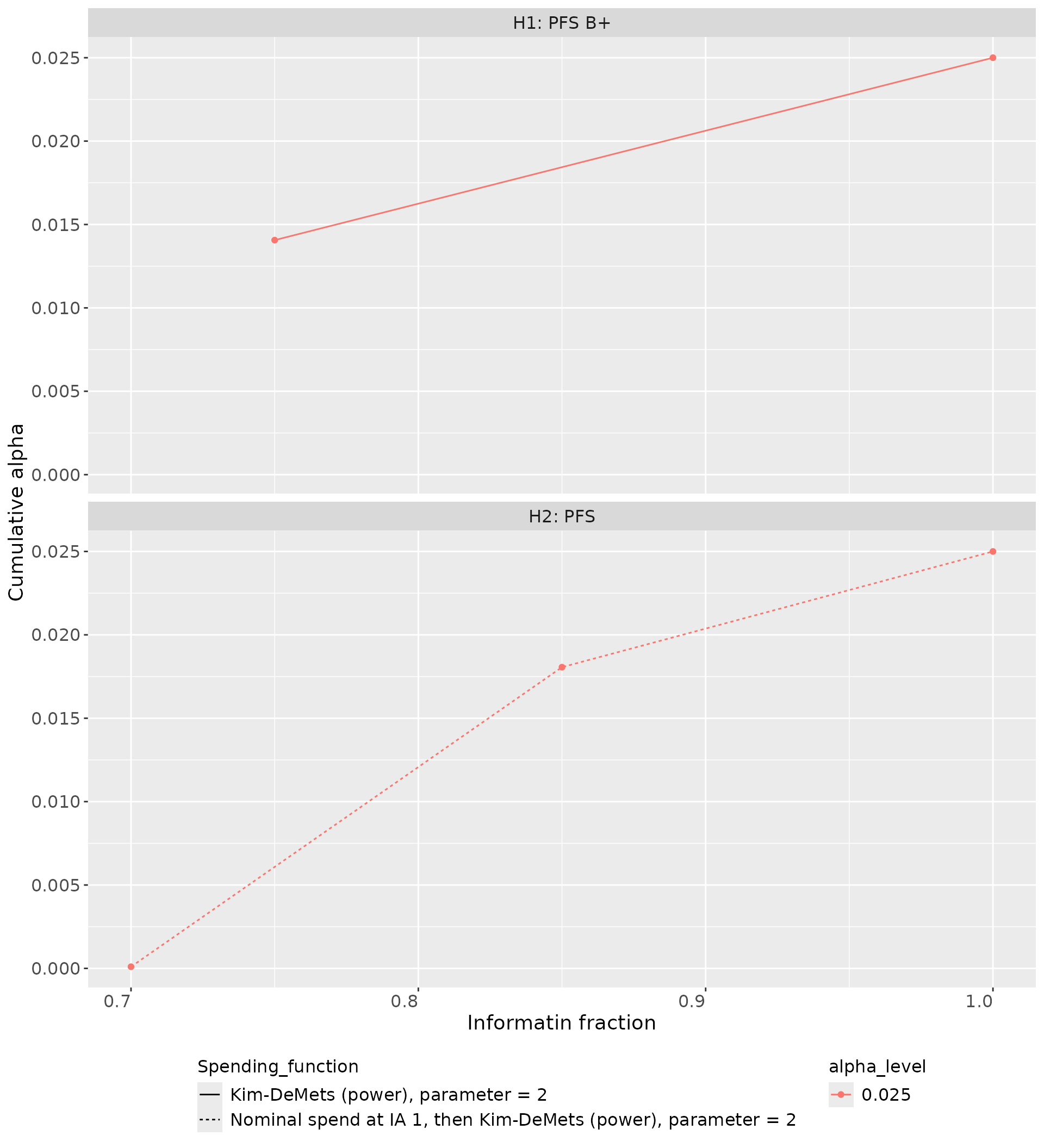
Alpha-spending functions